Introduction
If you ever had a probability course, it’s probably that you had to solve the birthday paradox (also called as the birthday problem) or had heard of it at least.
- The birthday paradox consists of measuring the probability of at least 2 persons in a room, with n < 365 persons, were born on the same day (\(p(n)\)).
- To calculate this is necessary to make the assumptions that are 365 possibilities of days and each day has the same probability of being a birthday.
Thinking on the complementary probability \(p^c(n)\)(probability of none of the persons had born on the same day), after some inspiration you get:
\(p^c(n) = 1 \times (1 - \frac{1}{365}) \times (1 - \frac{2}{365}) \times ... \times (1 - \frac{n-1}{365}) = \frac{365!}{365^n(365-n)!}\)
With more inspiration and some free time you can see that it can be approximated, by a Taylor expansion to:
\(p^c(n) \approx e^{-(n(n-1)) / 2 \times 365}\)
And then:
\(p(n) = 1 - p^c(n) \approx 1 - e^{-(n(n-1)) / 2 \times 365}\)
- But … What if you don’t want to do all the math by hand? Well, you can always (not always, but you get the point) simulate! So let’s do that in R!
Solving methods in R
- If you want, you can implement the (boring) analytic solution using:
library(tidyverse)
library(scales)

boring = function(n) 1 - exp(-(n*(n-1)) / (2 * 365))- The you can calculate using the function:
tibble(n = 1:23, p = percent(boring(1:23)))%>%
knitr::kable(align = "c")| n | p |
|---|---|
| 1 | 0.0% |
| 2 | 0.3% |
| 3 | 0.8% |
| 4 | 1.6% |
| 5 | 2.7% |
| 6 | 4.0% |
| 7 | 5.6% |
| 8 | 7.4% |
| 9 | 9.4% |
| 10 | 11.6% |
| 11 | 14.0% |
| 12 | 16.5% |
| 13 | 19.2% |
| 14 | 22.1% |
| 15 | 25.0% |
| 16 | 28.0% |
| 17 | 31.1% |
| 18 | 34.2% |
| 19 | 37.4% |
| 20 | 40.6% |
| 21 | 43.7% |
| 22 | 46.9% |
| 23 | 50.0% |
With 23 persons the probability is about 50%!
But… You can simulate, using the idea of frequentist probability, that is if you simulate a lot of rooms, let’s say 10000, then you count the number of rooms which the event happened, the proportion of occurrences will converge to the true probability of occurrence.
You can implement this in R using:
# Define the function
birthday = function(n){
# Create a empty vector
  y = NULL

# Simulate the 10000 rooms
  for (i in 1:10000) {

# Verify if at least 2 numbers match
    y[i] = length(table(sample(1:365,
                               size = n,
                               replace = T))) < n

  }

# Return the proportion
  return(mean(y))
}- And then you can use the function:
birthday(n = 23)## [1] 0.5078The results aren’t exactly equal but are close and can be even closer if the number of simulations increases.
To ilustrate, we can compare the curves of the analytical and the simulated solutions:
tibble(n=seq(1,60,by = 5),
       analytical = boring(seq(1,60,by = 5)),
       simulated = sapply(seq(1,60,by = 5),birthday))%>%
  gather("Method","Probability",-n)%>%
  ggplot(aes(n,Probability,col=Method))+
  geom_line(size=1.2)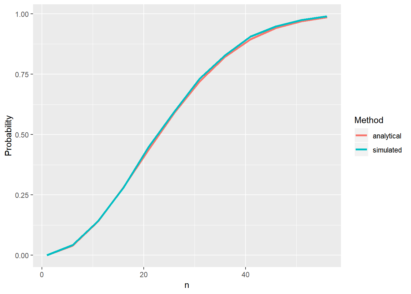
- Seems pretty ok…
The pRoblem with simulations
So, it’s known that R isn’t the fasted language to do loops like this one.
Thus, to solve the problem, we can try some methods. The first will be compile the function using a byte compiler:
library(compiler) #Package with the compiler function

comp.birthday = cmpfun(birthday,
                       options = list(optimize=3,
                                      enableJIT=3))
comp.birthday(n=23)
## [1] 0.5001- A more refined approach would be using parallel computing. In R, it’s pretty straightforward with the
foreachanddoParallelpackages.
library(foreach)
library(doParallel)

para.birthday = function(n){
#setup parallel backend
cores=detectCores()
cl <- makeCluster(cores[1]-1,useXDR=F)
registerDoParallel(cl)

# Parallel "for" loop
y = foreach(i=1:10000) %dopar% {

  length(table(sample(1:365,
                        size = n,
                        replace = T))) < n

}

# Closing clusters
stopCluster(cl)

# Returning the proportions
return(mean(unlist(y)))
}

para.birthday(n=23)
## [1] 0.5084But, how much faster did we get?
- To measure and compare the time of the 3 simulation methods, we can use each function a bunch of times and calcule the mean time of processing. Thankfully there is no need to do this “by hand” and it can be done with the
microbenchmarkpackage:
library(microbenchmark)

(bench.inf = microbenchmark(birthday(50),
                           comp.birthday(50),
                           para.birthday(50),
                           times = 30))
## Unit: seconds
## expr min lq mean median uq max
## birthday(50) 1.507785 1.535846 1.581197 1.571302 1.607885 1.832825
## comp.birthday(50) 1.509345 1.540851 1.565712 1.556180 1.581613 1.711634
## para.birthday(50) 6.589781 6.663439 6.797821 6.730544 6.971870 7.170535
## neval cld
## 30 a
## 30 a
## 30 bautoplot(bench.inf)## Coordinate system already present. Adding new coordinate system, which will replace the existing one.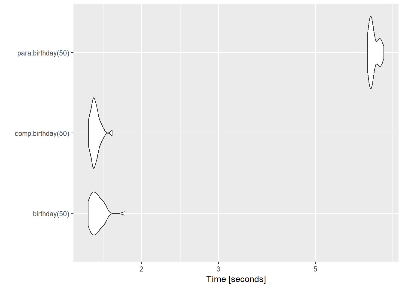
- It’s funny because the more complex solution (parallel computing) get the worst result by far.
- This happened for two main reasons:
We lost about 1 or 2 second just to setup the clusters;
The calculations are way too simply to worth the “parallelization”, that is, the time taken to split and pass the information for the cores is too much when compared to the real calculation made by the function.
- So, there is some methods to solve the birthday paradox!