Introduction
- Like almost everyone here in Brazil, I have a passion for football (or soccer) and because of that my father and I are always alert to the national championship.
So, a few days ago my father gave me a challenge, he challenged me to understand what is needed to be a champion in the brazilian national soccer league (knowed here as “Brasileirão”) since the competition change its format to a point based championship in 2003.
Thus I’ve accepted the challenge and here are the results:
Data
- Firstly we need to get the data!!
I haven’t found a well structured data base to work with, so I had to work with the information provided by this site and I had to do a function to scrap the data.
- Packages used
library(XML)      #Package to do web scraping
library(dplyr)    #Manipulation
library(magrittr) #Manipulation
library(tidyr)    #Manipulation
library(scales)   #Formatting
library(ggplot2)  #Plots
library(pROC) #ROC curves- That is the function to do the web scraping. Note that the site has information only until 2015.
# URL base to all years
url1="futpedia.globo.com/campeonato
/campeonato-brasileiro/"

#Empty data frame to store the information
games= data_frame()

for (i in 2003:2015) { ## years
  url2 = paste0(url1,i)

  readHTMLTable(url2,as.data.frame = T)%>%
    data.table::rbindlist()%>%
    setNames(c("Position","Team","Points","Games","Victories","Ties",
               "Losses","Goals scored","Goals conceded","Goal difference",
               "Performance"))%>%
    mutate(Year = i)%>%
    bind_rows(games) -> games
}
If you don’t want to scrap the data (because it can take some time and sometimes doesn’t work so fine) you can get it from here Data!.
Tip: Be aware with the encoding! (use “latin-1”)
- Moving on, we need some extra information, like which team was the champion in the season and how many games (rounds) are in each season, because the number of teams has changed in 2005 and changed again in 2006.
# Champions data
champ_dt = data_frame(Year = 2003:2018,
                      Champion = c("Cruzeiro","Santos","Corinthians","São Paulo",
                                   "São Paulo","São Paulo","Flamengo","Fluminense",
                                   "Corinthians","Fluminense","Cruzeiro","Cruzeiro",
                                   "Corinthians","Palmeiras","Corinthias","Palmeiras"))
games %<>% # Tracking the round (game) number
mutate(Round = c(rep(rep(1:38,each =20),10),
rep(1:42,each =22),
rep(1:46,each =24),rep(1:46,each =24)))%>%
# Finding the champion in each season
inner_join(champ_dt) %>%
# Is this team the champion of this year?
mutate(Champ = if_else(Team == Champion, 1,0),
# Total number of games in the season
N_round = case_when(Year < 2005 ~ 46,
Year == 2005 ~ 42,
Year > 2005 ~38),
# In this round, this team is in the first place?
First_place = if_else(Position ==1,1,0 ),
# In this round, this team is in the first place
# and is the champion?
TP = if_else(First_place == 1 & Champ == 1,
1,0),
# In this round, this team is in the first place
# and isn't the champion?
TN = if_else(First_place == 1 & Champ == 1,
1,0))- Let’s take a look in the data
head(games)## Position Team Points Games Victories Ties Losses Goals scored
## 1 1 Sport 3 1 1 0 0 4
## 2 2 Athletico-PR 3 1 1 0 0 3
## 3 3 Chapecoense 3 1 1 0 0 2
## 4 3 São Paulo 3 1 1 0 0 2
## 5 5 Corinthians 3 1 1 0 0 1
## 6 6 Fluminense 3 1 1 0 0 1
## Goals conceded Goal difference Performance Year Round Champion Champ
## 1 1 3 100 2015 1 Corinthians 0
## 2 0 3 100 2015 1 Corinthians 0
## 3 1 1 100 2015 1 Corinthians 0
## 4 1 1 100 2015 1 Corinthians 0
## 5 0 1 100 2015 1 Corinthians 1
## 6 0 1 100 2015 1 Corinthians 0
## N_round First_place TP TN
## 1 38 1 0 0
## 2 38 0 0 0
## 3 38 0 0 0
## 4 38 0 0 0
## 5 38 0 0 0
## 6 38 0 0 0All seems ok, let’s continue…
Analysing the initial rounds.
- So, now we can analyse the data. Initially, we can try to find the “champion profile” at the 5th and 10th round.
5th round:
# Making a plot
games %>%
  filter(Round == 5)%>%
  select(Points, Victories, Ties, Losses,
         `Goals scored`, `Goals conceded`,
         Position,Champ)%>%
  mutate_all(.funs = as.numeric)%>%
  mutate(Champ = factor(Champ, labels= c("Not champion","Champion")))%>%
  gather(key="Variable",value="value",-c(Champ))%>%
  group_by(Champ,Variable)%>%
  mutate(tot = n())%>%
  group_by(Champ,Variable,value)%>%
  summarise(freq = n(), tot=mean(tot))%>%
  mutate(perc = freq/tot)%>%
  ggplot(aes(value,perc,fill=Champ))+
  geom_col(width = 1,col=1,alpha=.3)+
  facet_wrap(~Variable,scales = "free")+
  theme_light()+
  scale_fill_discrete("")+
  ylab("Frequency (%)")+
  scale_y_continuous(labels = scales::percent)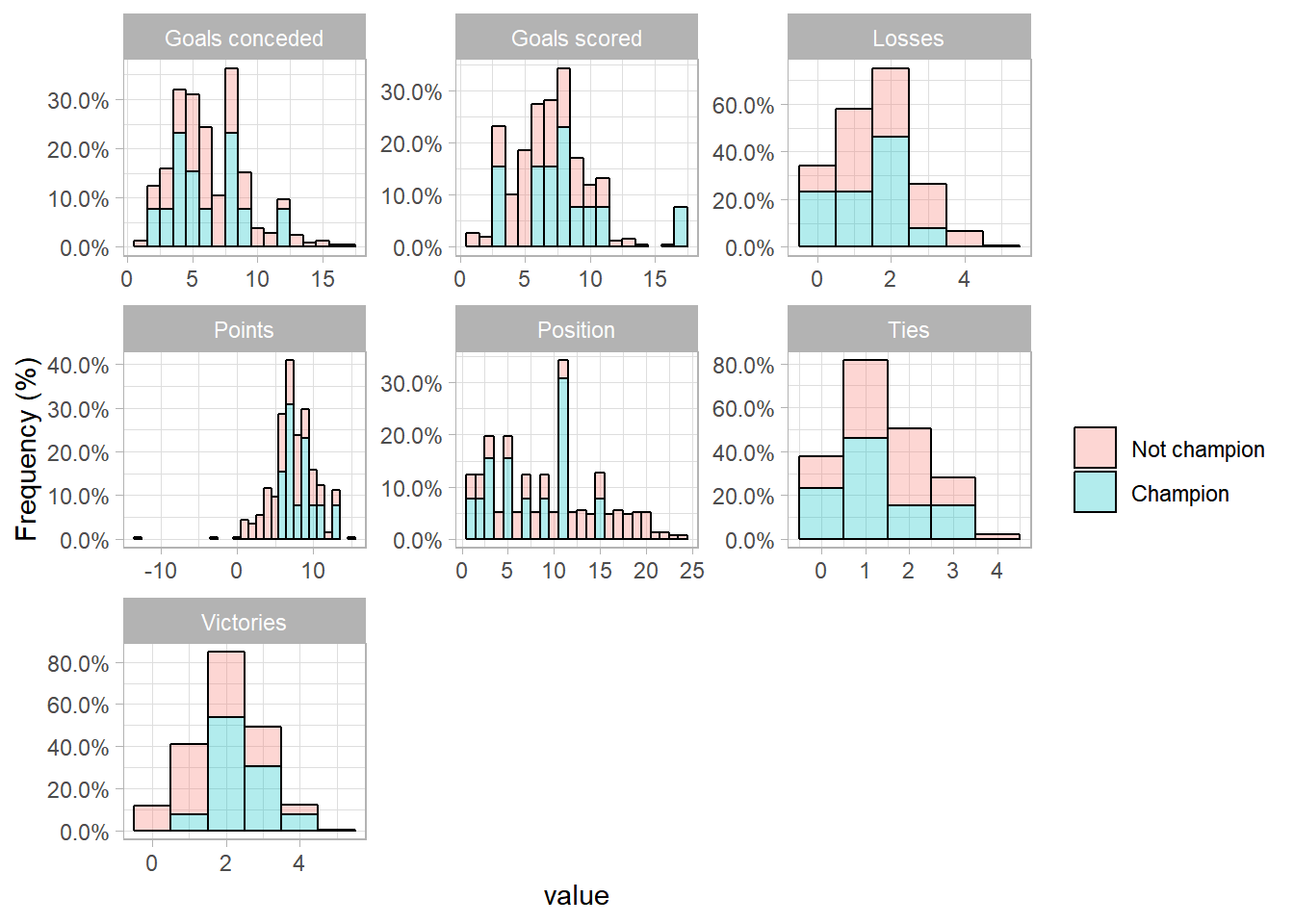
- Note that are negative points, this happened because of punishments gave by CBF for some teams.
# Making a table
games %>%
  filter(Round == 5)%>%
  select(Points, Victories, Ties, Losses,
         `Goals scored`, `Goals conceded`,
         Position,Champ,Performance)%>%
  mutate_all(.funs = as.numeric)%>%
  mutate(Champ = factor(Champ, labels= c("Not champion","Champion")))%>%
  gather(key="Variable",value="value",-c(Champ))%>%
  group_by(Variable,Champ)%>%
  summarise(Min= min(value),
            Mean = mean(value) %>% round(digits = 2),
            Max = max(value),
            SD = sd(value) %>% round(digits = 2))%>%
knitr::kable()| Variable | Champ | Min | Mean | Max | SD |
|---|---|---|---|---|---|
| Goals conceded | Not champion | 1 | 6.59 | 17.0 | 2.95 |
| Goals conceded | Champion | 2 | 6.00 | 12.0 | 2.83 |
| Goals scored | Not champion | 1 | 6.49 | 16.0 | 2.71 |
| Goals scored | Champion | 3 | 7.92 | 17.0 | 3.59 |
| Losses | Not champion | 0 | 1.77 | 5.0 | 1.10 |
| Losses | Champion | 0 | 1.38 | 3.0 | 0.96 |
| Performance | Not champion | 0 | 44.44 | 100.0 | 19.67 |
| Performance | Champion | 40 | 55.91 | 86.7 | 13.75 |
| Points | Not champion | -13 | 6.57 | 15.0 | 3.26 |
| Points | Champion | 6 | 8.38 | 13.0 | 2.06 |
| Position | Not champion | 1 | 11.11 | 24.0 | 6.11 |
| Position | Champion | 1 | 7.23 | 15.0 | 4.40 |
| Ties | Not champion | 0 | 1.52 | 4.0 | 0.96 |
| Ties | Champion | 0 | 1.23 | 3.0 | 1.01 |
| Victories | Not champion | 0 | 1.72 | 5.0 | 1.07 |
| Victories | Champion | 1 | 2.38 | 4.0 | 0.77 |
Here we can see that, at the 5th round, all the champions have woned at least one game, and drawn three games at the most, with the minimum performance (points made / possible points) of 40%, but none of the champions had a performance score of 100% at the 5th round.
The minimum number of goals scored by the champions was 3 and the maximum number of goals conceded was 12.
10th round:
# Making a plot
games %>%
  filter(Round == 10)%>%
  select(Points, Victories, Ties, Losses,
         `Goals scored`, `Goals conceded`,
         Position,Champ)%>%
  mutate_all(.funs = as.numeric)%>%
  mutate(Champ = factor(Champ, labels= c("Not champion","Champion")))%>%
  gather(key="Variable",value="value",-c(Champ))%>%
  mutate(y = if_else(Champ=="Champion", value/13,value/ 270 ))%>%
  ggplot(aes(value,fill=Champ))+
  #geom_point()+
  geom_histogram(aes(y=..density..),binwidth = 1,col=1,alpha=.3)+
  facet_wrap( ~Variable,scales = "free")+
  theme_light()+
  scale_fill_discrete("")+
  ylab("Frequency (%)")+
  scale_y_continuous(labels = scales::percent)+
  scale_x_continuous(breaks = seq(0,30,by=4))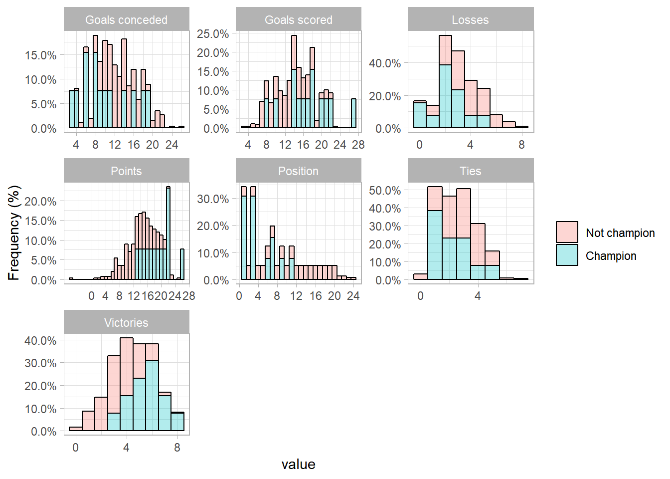
- Note that are negative points again, this happened because of the same reason.
# Making a table
games %>%
  filter(Round == 10)%>%
  select(Points, Victories, Ties, Losses,
         `Goals scored`, `Goals conceded`,
         Position,Champ,Performance)%>%
  mutate_all(.funs = as.numeric)%>%
  mutate(Champ = factor(Champ, labels= c("Not champion","Champion")))%>%
  gather(key="Variable",value="value",-c(Champ))%>%
  group_by(Variable,Champ)%>%
  summarise(Min= min(value),
            Mean = mean(value) %>% round(digits = 2),
            Max = max(value),
            SD = sd(value)%>% round(digits = 2))%>%
knitr::kable()| Variable | Champ | Min | Mean | Max | SD |
|---|---|---|---|---|---|
| Goals conceded | Not champion | 4.0 | 13.30 | 26.0 | 3.89 |
| Goals conceded | Champion | 3.0 | 10.15 | 19.0 | 5.19 |
| Goals scored | Not champion | 3.0 | 12.95 | 23.0 | 3.95 |
| Goals scored | Champion | 8.0 | 16.92 | 27.0 | 5.04 |
| Losses | Not champion | 0.0 | 3.66 | 8.0 | 1.62 |
| Losses | Champion | 0.0 | 2.23 | 5.0 | 1.42 |
| Performance | Not champion | 6.7 | 44.42 | 83.3 | 14.16 |
| Performance | Champion | 43.3 | 62.82 | 86.7 | 12.61 |
| Points | Not champion | -6.0 | 13.23 | 25.0 | 4.48 |
| Points | Champion | 13.0 | 18.85 | 26.0 | 3.78 |
| Position | Not champion | 1.0 | 11.27 | 24.0 | 6.02 |
| Position | Champion | 1.0 | 4.31 | 11.0 | 3.35 |
| Ties | Not champion | 0.0 | 2.84 | 7.0 | 1.31 |
| Ties | Champion | 1.0 | 2.23 | 5.0 | 1.30 |
| Victories | Not champion | 0.0 | 3.49 | 8.0 | 1.51 |
| Victories | Champion | 3.0 | 5.54 | 8.0 | 1.39 |
In the 10th round we can see that the champions scored at least 8 goals, conceded at least 3 goals and lose 5 games at the most. We can see also that all the champions have woned at least 3 games, and drawn between one and five games, with the minimum performance (points made / possible points) of 43.3%.
How many rounds on top make a champion?
So, to answer my dad’s question about the football champions I thought that discovery the numbers of rounds in the first place would be of great value.
- Thus now we need to count the number of rounds in first place of each team in each season (year).
games %>%
  group_by(Year,Team)%>%
  #Counting the number of rounds on top
  summarise(Rounds_on_top = sum(First_place))%>%
  inner_join(champ_dt)%>%
  #Was this team the champion of the season?
  mutate(Won = (Team==Champion),
         Won = as.numeric(Won),
         N_round = case_when(Year < 2005 ~ 46,
                             Year == 2005 ~ 42,
Year > 2005 ~38)) -> first_place_df- We can now calcule the proportions of rounds needed.
first_place_df%>%
  mutate(Proportion = Rounds_on_top/N_round,
         Won = factor(Won,labels = c("Not champion",
                                 "Champion")))%>%
  ggplot(aes(Proportion))+
  geom_histogram(bins = 5,col=1,alpha=.5)+
  facet_wrap(~Won,scales = "free_y")+
  theme_light()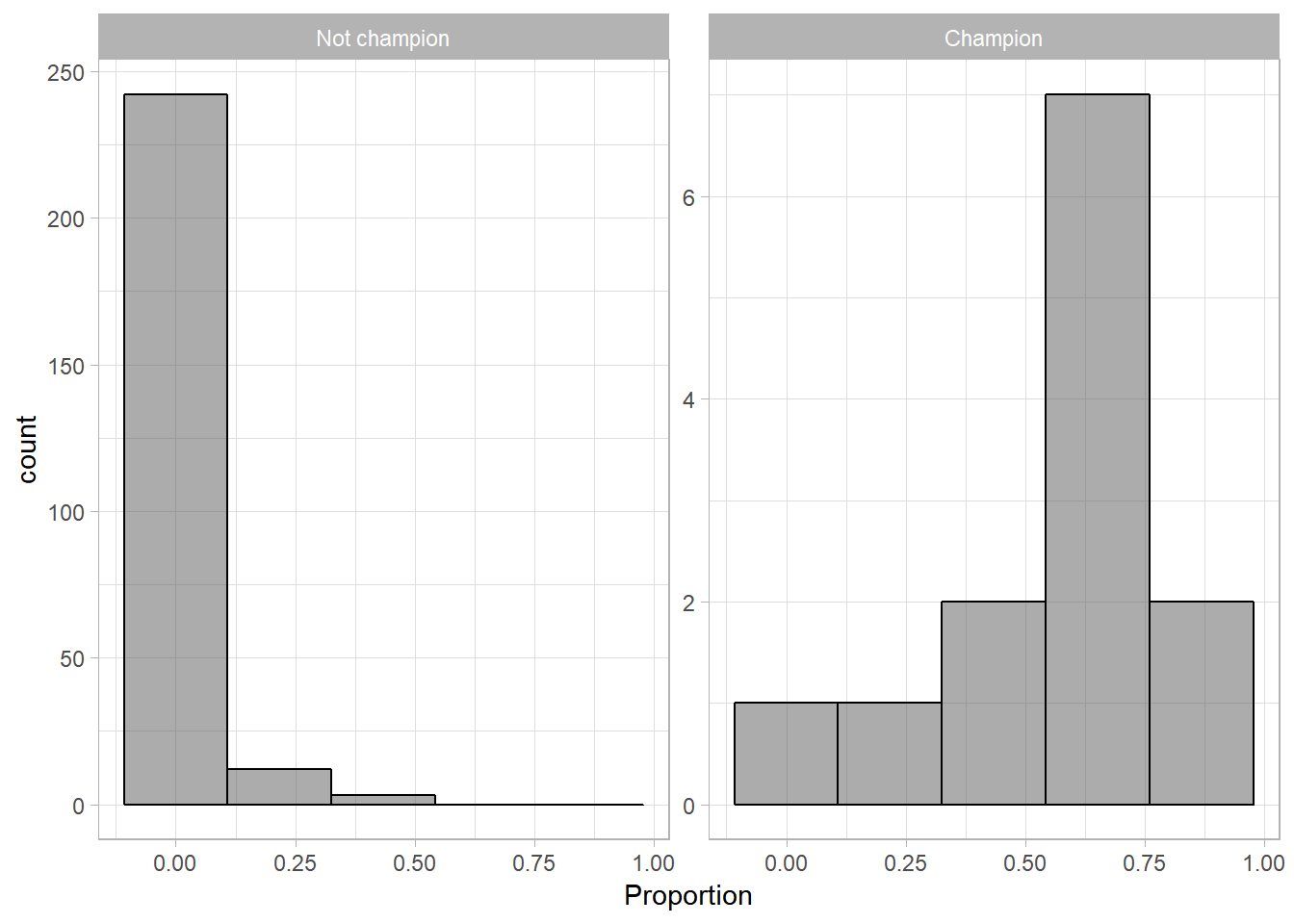
first_place_df%>%
  mutate(Proportion = Rounds_on_top/N_round,
         Won = factor(Won,labels = c("Not champion",
                                 "Champion")))%>%
  group_by(Won)%>%
  summarise(min_n=min(Rounds_on_top) %>% round(digits = 2),
            mean_n = mean(Rounds_on_top) %>% round(digits = 2),
            max_n=max(Rounds_on_top) %>% round(digits = 2),
            min_prop=min(Proportion) %>% percent(),
            mean_prop = mean(Proportion) %>% percent(),
            max_prop=max(Proportion) %>% percent())%>%
knitr::kable()| Won | min_n | mean_n | max_n | min_prop | mean_prop | max_prop |
|---|---|---|---|---|---|---|
| Not champion | 0 | 0.89 | 17 | 0% | 2.27% | 44.7% |
| Champion | 2 | 22.38 | 38 | 5.26% | 56.4% | 86.8% |
- So, we can note that the minimum number of rounds on top was 2 (Flamengo, 2009), while the maximum number was 38 (Cruzeiro, 2003) and the average was about 22 games. Looking on the proportions, we can see that the champions often stays on the top a bit more than half of the championship (56,4%).
Estimating the number of rounds
- To estimate the number of rounds, we can consider a logist regression with “champion” (binary) as the response variable and the proportion of rounds on first as the predictor variable.
first_place_df%<>%
  mutate(Proportion = Rounds_on_top/N_round)

#fitting the model

fit=glm(Won ~ Proportion,
        family = binomial(link = "logit"),
        data=first_place_df)

summary(fit)
##
## Call:
## glm(formula = Won ~ Proportion, family = binomial(link = "logit"),
## data = first_place_df)
##
## Deviance Residuals:
## Min 1Q Median 3Q Max
## -1.30508 -0.08386 -0.08386 -0.08386 3.14843
##
## Coefficients:
## Estimate Std. Error z value Pr(>|z|)
## (Intercept) -5.6485 0.9264 -6.097 1.08e-09 ***
## Proportion 13.2860 2.5762 5.157 2.51e-07 ***
## ---
## Signif. codes: 0 '***' 0.001 '**' 0.01 '*' 0.05 '.' 0.1 ' ' 1
##
## (Dispersion parameter for binomial family taken to be 1)
##
## Null deviance: 104.234 on 269 degrees of freedom
## Residual deviance: 28.442 on 268 degrees of freedom
## AIC: 32.442
##
## Number of Fisher Scoring iterations: 8Obviously the proportion of rounds in first is a important variable to explain the win. Let’s take a look in the ROC curve.
(ROC = roc(Won ~ Proportion,data=first_place_df,percent=T))##
## Call:
## roc.formula(formula = Won ~ Proportion, data = first_place_df, percent = T)
##
## Data: Proportion in 257 controls (Won 0) < 13 cases (Won 1).
## Area under the curve: 98.59%ggroc(ROC)+
theme_light()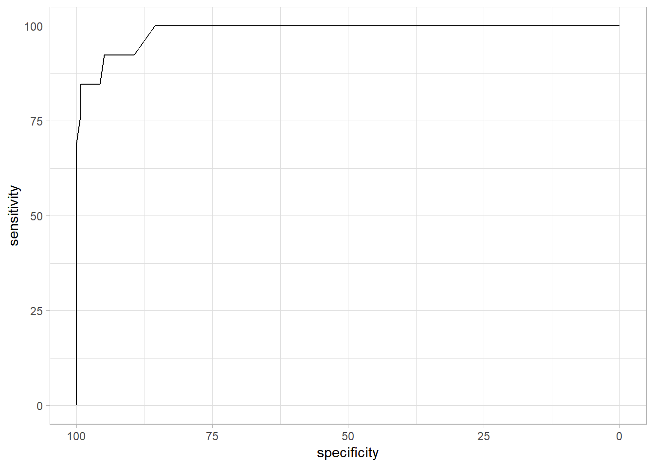
- We got 98.59% of Area under the curve (which is excellent). Now we can look on the true positive ratio and true negative ratio to decide a cut point.
data_frame(Proportion = ROC$thresholds,
           Sens = ROC$sensitivities %>% round(digits = 2),
           Speci = ROC$specificities %>% round(digits = 2))%>%
  mutate(Proportion = percent(Proportion))%>%
knitr::kable()| Proportion | Sens | Speci |
|---|---|---|
| -Inf | 100.00 | 0.00 |
| 1.1% | 100.00 | 77.04 |
| 2.3% | 100.00 | 78.21 |
| 2.5% | 100.00 | 79.38 |
| 3.5% | 100.00 | 84.44 |
| 4.6% | 100.00 | 85.21 |
| 5.0% | 100.00 | 85.60 |
| 5.9% | 92.31 | 89.49 |
| 7.2% | 92.31 | 90.66 |
| 8.3% | 92.31 | 92.61 |
| 9.1% | 92.31 | 93.00 |
| 10.0% | 92.31 | 93.39 |
| 10.7% | 92.31 | 94.16 |
| 12.0% | 92.31 | 94.55 |
| 14.5% | 92.31 | 94.94 |
| 17.1% | 84.62 | 95.72 |
| 18.7% | 84.62 | 96.50 |
| 20.1% | 84.62 | 96.89 |
| 21.4% | 84.62 | 97.28 |
| 24.0% | 84.62 | 97.67 |
| 27.6% | 84.62 | 98.05 |
| 30.3% | 84.62 | 98.44 |
| 35.5% | 84.62 | 98.83 |
| 41.5% | 84.62 | 99.22 |
| 44.1% | 76.92 | 99.22 |
| 51.3% | 69.23 | 100.00 |
| 59.2% | 53.85 | 100.00 |
| 61.2% | 46.15 | 100.00 |
| 66.5% | 38.46 | 100.00 |
| 72.4% | 23.08 | 100.00 |
| 78.1% | 15.38 | 100.00 |
| 84.7% | 7.69 | 100.00 |
| Inf | 0.00 | 100.00 |
Seems like 41,5% is an good cut point because we got 99,22% of specifity (probability of classify the true champion as champion) without losing so much sensibility.
So let’s take a look on the model results…
data_frame(Proportion=seq(0,1,by=.05),
           prob=predict(fit,
                        newdata = data_frame(Proportion=seq(0,1,by=.05)),
                        type = "response")
)%>%
  mutate(prob = percent(prob))%>%
knitr::kable()| Proportion | prob |
|---|---|
| 0.00 | 0.4% |
| 0.05 | 0.7% |
| 0.10 | 1.3% |
| 0.15 | 2.5% |
| 0.20 | 4.8% |
| 0.25 | 8.9% |
| 0.30 | 15.9% |
| 0.35 | 26.9% |
| 0.40 | 41.7% |
| 0.45 | 58.2% |
| 0.50 | 73.0% |
| 0.55 | 84.0% |
| 0.60 | 91.1% |
| 0.65 | 95.2% |
| 0.70 | 97.5% |
| 0.75 | 98.7% |
| 0.80 | 99.3% |
| 0.85 | 99.6% |
| 0.90 | 99.8% |
| 0.95 | 99.9% |
| 1.00 | 100.0% |
Finnaly I can answer to my dad what is the estimated probability of a team be the champion based on how many rounds it was in the first place!